Three Dimensional objects representation in computer graphics

In graphic scenes, there are various objects such as trees, flowers, clouds, rocks, water, bricks, wood paneling, rubber, paper, marble, steel, glass, plastic, and cloth. Due to the diverse nature of these materials, there is no single method that can encompass all their characteristics. To create realistic displays of scenes, we need accurate representations that can model the specific characteristics of objects.

There are different approaches to describing objects depending on their properties. For simple geometric objects like polyhedrons and ellipsoids, polygon and quadric surfaces provide precise descriptions. Spline surfaces and construction techniques are useful for designing curved surfaces found in aircraft wings, gears, and other engineering structures. Procedural methods, such as fractal constructions and particle systems, allow us to accurately represent natural objects like clouds and clumps of grass. Physically based modeling methods employ systems of interacting forces to describe the non-rigid behavior of objects like cloth or gelatin. Octree encodings are used to represent the internal features of objects, particularly those obtained from medical CT images. Visualization techniques like isosurface displays, volume renderings, and others are applied to three-dimensional data sets to obtain visual representations of the data.

Representation schemes for solid objects are often categorized into two main types, although not all representations strictly fall into one category. Boundary representations (B-reps) describe a three-dimensional object as a collection of surfaces that separate the object’s interior from the surrounding environment. Examples of boundary representations include polygon facets and spline patches. On the other hand, space-partitioning representations are used to describe interior properties by dividing the spatial region containing an object into small, non-overlapping, contiguous solids, often cubes. An example of a space-partitioning description is an octree representation. This article explores the features of these different representation schemes and how they are utilized in various applications.

POLYGON SURFACES

Polygon surfaces are a type of representation used to describe objects in computer graphics. They provide a precise and efficient way to represent simple geometric shapes, such as polyhedrons, in a three-dimensional space.

A polygon is a flat, two-dimensional shape with straight sides, typically forming a closed loop. In the context of computer graphics, polygons are often used as building blocks to construct more complex three-dimensional objects.

To create a polygon surface, a set of vertices (points in space) are connected by straight edges to form a closed polygonal shape. The polygons can have any number of sides, but triangles (three-sided polygons) and quadrilaterals (four-sided polygons) are the most commonly used.

The vertices of the polygons define the shape and structure of the object. By specifying the coordinates of these vertices in three-dimensional space, we can determine the position, size, and orientation of the object. Additionally, attributes such as color, texture, and surface normals can be associated with each vertex to provide visual details and shading information.

Polygon surfaces are widely used in computer graphics due to their simplicity and efficiency in rendering. They can accurately represent many basic shapes and can be easily manipulated, transformed, and rendered using algorithms and techniques such as rasterization and shading.

However, polygon surfaces have certain limitations. They are best suited for representing objects with flat or planar surfaces and may not be suitable for objects with complex curved or organic shapes. In such cases, more advanced techniques like spline surfaces or procedural methods may be employed.

Overall, polygon surfaces play a fundamental role in computer graphics, providing a versatile and widely adopted representation for rendering and visualizing three-dimensional objects.

Polygon Tables

Polygon tables are data structures used in computer graphics to store information about polygons in a scene. They provide a systematic way to organize and manage polygon data for efficient rendering and manipulation.

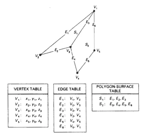
A polygon table typically consists of a collection of records, with each record representing a single polygon in the scene. Each record in the table contains various attributes and information associated with the corresponding polygon, such as the vertices, surface normals, texture coordinates, and other relevant properties.

The polygon table allows for easy access and retrieval of polygon data during rendering and other graphics operations. It serves as a central repository for all the necessary information needed to render the polygons accurately on the screen.

One of the key components of a polygon table is the vertex list, which stores the coordinates of the vertices that define each polygon. The vertex list ensures that the correct position and shape of the polygons are maintained. Additionally, the table may contain information about the connectivity between vertices to form polygons, such as edge lists or face lists.

In addition to vertex data, polygon tables often include other attributes for each polygon. This can include surface normals, which specify the orientation of the polygon with respect to lighting calculations, and texture coordinates, which map textures onto the polygon’s surface.

Polygon tables are essential for efficient rendering algorithms like rasterization or ray tracing. They allow the graphics system to quickly access and process polygon data, enabling fast and accurate display of the scene on the screen.

Overall, polygon tables are a vital data structure in computer graphics, providing a systematic way to organize and manage polygon data for efficient rendering and manipulation of three-dimensional scenes.

Plane Equations

Plane equations are mathematical representations used to describe a plane in three-dimensional space. They provide a concise and precise way to define a flat surface that extends infinitely in all directions.

A plane equation is typically expressed in the form of:

Ax + By + Cz + D = 0

In this equation, A, B, and C represent the coefficients of the variables x, y, and z, respectively. They determine the orientation and direction of the plane in relation to the coordinate system. The coefficient D is a constant term that affects the position of the plane along the normal vector.

The coefficients A, B, and C can be interpreted as the components of a normal vector to the plane. The normal vector is perpendicular to the plane and determines its orientation. By knowing the direction of the normal vector, we can determine which side of the plane is considered the front or back.

The values of A, B, C, and D in the plane equation can be determined using different methods. For example, if we know three non-collinear points that lie on the plane, we can use those points to calculate the coefficients. Alternatively, if we know the normal vector and a point on the plane, we can derive the coefficients using vector operations.

Once the coefficients are known, the plane equation can be used for various purposes in computer graphics and geometry. It allows us to perform operations such as determining whether a point lies on the plane, calculating the distance between a point and the plane, or finding the intersection of multiple planes.

Plane equations are widely used in computer graphics applications such as rendering, collision detection, and geometric modeling. They provide a convenient mathematical representation for defining and working with flat surfaces in three-dimensional space.

The equation of a plane can be represented using a matrix equation. Let’s consider a plane defined by the normal vector [A, B, C] and a point on the plane [x₀, y₀, z₀]. The equation of the plane can be expressed as:

[A B C] ⋅ [x – x₀, y – y₀, z – z₀] = 0

In this equation, [x, y, z] represents a point in three-dimensional space. The expression [x – x₀, y – y₀, z – z₀] represents the vector from the given point on the plane [x₀, y₀, z₀] to the point [x, y, z]. The dot product of the normal vector [A, B, C] and the vector [x – x₀, y – y₀, z – z₀] is taken, and the result is set equal to zero.

This matrix equation provides a concise representation of the plane equation. It allows us to perform computations efficiently, such as determining whether a point lies on the plane or finding the distance between a point and the plane.

Note that in this matrix equation, the normal vector [A, B, C] represents the coefficients of the plane equation, and the point [x₀, y₀, z₀] represents a known point on the plane. By manipulating the matrix equation, we can derive different forms of the plane equation, such as the general form Ax + By + Cz + D = 0, where D is a constant term.

Matrices provide a powerful tool for representing and manipulating mathematical equations, including plane equations, in a compact and efficient manner.

Polygon Meshes

Polygon meshes are widely used in computer graphics to represent complex three-dimensional objects. They are composed of a collection of polygons that are connected together to form a mesh-like structure.

In a polygon mesh, each polygon is typically a triangle or a quadrilateral, although other polygon types can also be used. The polygons share edges and vertices, creating a network of interconnected faces. This connectivity information allows for efficient representation and manipulation of the object’s surface.

Vertices play a crucial role in polygon meshes. They define the individual points in three-dimensional space that make up the object’s surface. Edges connect pairs of vertices, forming the boundaries of polygons. The polygons themselves define the flat faces of the mesh.

Polygon meshes provide flexibility in representing objects with various shapes and surface details. By using polygons of different sizes and arrangements, meshes can capture the complexity of real-world objects with irregular surfaces.

The level of detail in a polygon mesh can vary based on the application and desired visual fidelity. High-resolution meshes consist of many small polygons, resulting in a more accurate representation of the object’s shape. On the other hand, low-resolution meshes use larger polygons, providing a simplified representation suitable for real-time applications or when computational resources are limited.

Polygon meshes offer several advantages in computer graphics. They are versatile, allowing for efficient rendering, collision detection, and other computations. They also support various operations, such as smoothing, subdivision, and deformation, enabling artists and designers to manipulate the shape and appearance of objects.

However, polygon meshes also have limitations. They may struggle to accurately represent objects with highly curved or organic surfaces, requiring a large number of polygons to approximate the shape faithfully. Additionally, meshes can introduce artifacts like gaps or self-intersections if not constructed or processed carefully.

Overall, polygon meshes are a fundamental representation in computer graphics, enabling the creation and manipulation of complex three-dimensional objects. They serve as the foundation for many modeling, simulation, and rendering techniques used in various applications, including gaming, animation, virtual reality, and computer-aided design.

BLOBBY OBJECTS

Blobby objects, also known as metaballs or soft objects, are three-dimensional shapes that exhibit smooth and deformable properties. They are commonly used in computer graphics and modeling to represent objects with fluid-like or organic characteristics.

The concept of blobby objects can be understood through mathematical concepts such as implicit surfaces and distance functions. Implicit surfaces describe shapes based on a mathematical equation that defines whether a point in space is inside or outside the surface.

Blobby objects are often represented using implicit surfaces, where the equation determines the influence or contribution of nearby points or “blobs” to the shape of the object. Each blob has a position, radius, and influence on the surface based on its proximity to other blobs.

To determine if a point is inside or outside the blobby object, a distance function is used. The distance function measures the distance from the point to the nearest point on the surface of the object. If the distance is less than a certain threshold, the point is considered inside the object; otherwise, it is outside.

Blobby objects can exhibit various properties based on the underlying mathematical equations and distance functions. For example, by adjusting the radius and influence of each blob, the object can appear smooth or have sharp features. Additionally, manipulating the position and density of the blobs allows for deformation and dynamic changes in the shape of the object.

Metaballs, a specific type of blobby object, use a distance function based on the concept of a potential field. The potential field determines the strength of attraction or repulsion between blobs. As blobs come closer together, the potential field increases, causing the object to merge or form interconnected regions.

Blobby objects provide a flexible and intuitive way to model complex and organic shapes. They are commonly used in applications such as character animation, fluid simulation, medical visualization, and special effects. Techniques like marching cubes or ray marching are often employed to render and visualize blobby objects efficiently.

Blobby objects can be mathematically represented using techniques such as Signed Distance Functions (SDFs) or Implicit Functions. These representations allow for the definition and manipulation of smooth, deformable objects with fluid-like or organic characteristics.

One common mathematical representation for blobby objects is the use of Signed Distance Functions (SDFs). An SDF assigns a signed distance value to every point in space, indicating the distance to the nearest point on the surface of the object. The sign of the distance value indicates whether the point is inside or outside the object.

Mathematically, an SDF for a blobby object can be represented as:

f(x, y, z) = c1/(|P1 – (x, y, z)|) + c2/(|P2 – (x, y, z)|) + … + cn/(|Pn – (x, y, z)|) – r

In this representation, (x, y, z) represents a point in three-dimensional space, P1, P2, …, Pn represent the positions of individual blobs, c1, c2, …, cn are coefficients representing the influence of each blob, and r is a radius parameter.

The SDF combines the influence of each blob by summing the reciprocal of the distance between the point and each blob’s position. The radius parameter controls the size of the blobs and determines the region of influence around each blob.

By evaluating the SDF at a specific point, we can determine its signed distance to the surface of the blobby object. Points with negative distances lie inside the object, points with positive distances lie outside the object, and points with a distance of zero lie precisely on the object’s surface.

Implicit Functions can also be used to represent blobby objects. An implicit function defines a level set where the function value is zero, representing the surface of the object. By evaluating the implicit function at a point, we can determine whether it lies inside or outside the object.

Mathematically, an implicit function for a blobby object can be represented as:

F(x, y, z) = c1 * phi(|P1 – (x, y, z)|) + c2 * phi(|P2 – (x, y, z)|) + … + cn * phi(|Pn – (x, y, z)|) – r

Here, phi(r) is a smooth function that determines the influence of each blob based on its distance to the point (x, y, z). The coefficients c1, c2, …, cn control the strength of influence of each blob, and r represents the radius of the blobs.

The implicit function F(x, y, z) provides a zero-crossing surface, where points with F(x, y, z) = 0 lie on the surface of the blobby object.

These mathematical representations of blobby objects using SDFs or Implicit Functions allow for the creation and manipulation of smooth, deformable objects with fluid-like or organic characteristics in computer graphics and modeling.

SPLINE REPRESENTATIONS

Spline representations are widely used in computer graphics and geometric modeling to describe smooth curves and surfaces. Splines provide a flexible and efficient way to approximate complex shapes and achieve smoothness in the representation of objects.

A spline is a mathematical curve or surface defined by a set of control points and interpolation or approximation algorithms. The control points act as anchors that guide the shape of the spline. By manipulating the positions and weights of these control points, various shapes can be achieved.

There are different types of splines used for different purposes, such as B-splines, NURBS (Non-Uniform Rational B-Splines), Bezier curves, and spline interpolation. Each type has its own characteristics and mathematical properties.

B-splines (Basis splines) are commonly used for curve and surface representation. They are defined by a set of control points and basis functions that determine the shape and smoothness of the curve or surface. B-splines allow for local control, meaning that changing the position of a control point affects only a local portion of the curve or surface.

NURBS are an extension of B-splines and provide additional flexibility by introducing weights to control points. These weights allow for precise control over the shape of the curve or surface, including the ability to represent conic sections such as circles and ellipses. NURBS are widely used in computer-aided design (CAD) and computer graphics applications due to their versatility and accuracy.

Bezier curves are another type of spline representation commonly used for smooth curve generation. They are defined by a set of control points that influence the shape of the curve. Bezier curves are known for their simplicity and ease of use, making them popular in graphics software for designing curves and paths.

Spline interpolation is a technique that involves constructing a smooth curve or surface that passes through a given set of data points. It is often used for data visualization and curve fitting applications. Spline interpolation ensures that the resulting curve or surface passes exactly through the specified points, maintaining smoothness and continuity.

Spline representations offer advantages such as flexibility, smoothness, and local control, making them valuable tools in computer graphics, geometric modeling, animation, and CAD. They enable artists, designers, and engineers to create and manipulate curves and surfaces with precision and aesthetic appeal.

BEZIER CURVES AND SURFACES

Bezier curves and surfaces are mathematical representations commonly used in computer graphics and geometric modeling to create smooth and visually appealing curves and surfaces. They provide a flexible and intuitive way to define and manipulate shapes, making them widely utilized in various applications.

Bezier Curves:
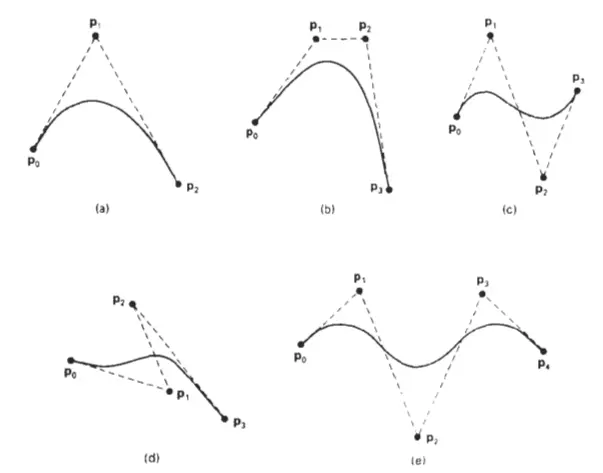
Bezier curves are defined by a set of control points that determine the shape of the curve. The curve starts at the first control point, ends at the last control point, and smoothly interpolates between them. The intermediate points influence the curve’s direction and curvature.

The shape of a Bezier curve is controlled by the blending of these control points through Bernstein polynomials. Each control point is multiplied by a specific Bernstein polynomial term, and their contributions are summed to determine the position of any point along the curve.

Bezier curves have several important properties, including local control, meaning that moving a control point affects only the nearby portion of the curve. They are also parameterized, meaning that they can be represented as a function of a parameter, usually denoted by t, allowing for easy evaluation of points along the curve.

Bezier Surfaces:
Bezier surfaces extend the concept of Bezier curves to two dimensions, creating smooth and continuous surfaces. They are defined by a grid of control points in a two-dimensional space. The control points define the corners and influence the shape of the surface.

Similar to Bezier curves, the blending of control points is achieved using Bernstein polynomials. The surface is formed by smoothly interpolating between the control points in both the u and v directions. By varying the positions of the control points, complex surface shapes can be created.

Bezier surfaces offer properties such as local control, allowing for precise manipulation of surface features. They can be evaluated at any point in the parameter space defined by u and v coordinates, making them suitable for both analytical calculations and rendering algorithms.

Applications of Bezier curves and surfaces are vast and include computer-aided design (CAD), 3D modeling, animation, and image editing. They provide a powerful and intuitive tool for artists, designers, and engineers to create smooth curves and surfaces with precise control over their shapes and characteristics.

Properties of Bkier Curves

Bezier curves possess several properties that make them useful and versatile in computer graphics and geometric modeling. Here are some key properties of Bezier curves:

1. Control Point Influence: The shape of a Bezier curve is determined by the positions of its control points. Each control point has an influence on the curve, affecting its direction and curvature. Moving a control point alters the shape of the curve locally, allowing for intuitive manipulation and control.
2. Local Control: Bezier curves exhibit local control, meaning that modifying the position of a control point affects only the nearby portion of the curve. Changes made to one segment of the curve do not impact the rest of the curve, facilitating precise adjustments.
3. Endpoint Interpolation: Bezier curves always start at the first control point and end at the last control point. This property guarantees that the curve passes through these endpoints, ensuring precise control over the curve’s path.
4. Parameterization: Bezier curves are parameterized, meaning that they can be expressed as a function of a parameter, commonly denoted as t. By varying the parameter t within the interval [0, 1], points along the curve can be evaluated. This enables easy interpolation and sampling of points on the curve.
5. Smoothness: Bezier curves exhibit smoothness, meaning they lack abrupt changes in direction or curvature. The blending of control points using Bernstein polynomials ensures a continuous and visually pleasing curve. Higher-degree Bezier curves tend to offer increased smoothness and flexibility.
6. Convex Hull Property: The curve lies entirely within the convex hull formed by its control points. This property guarantees that the Bezier curve remains within the boundary defined by its control points, making it suitable for various geometric operations.
7. Affine Invariance: Bezier curves maintain their shape under affine transformations such as translation, rotation, scaling, and shear. This property allows for easy manipulation and transformation of Bezier curves without altering their essential characteristics.
8. Degree Flexibility: Bezier curves can have different degrees, indicating the number of control points involved. Higher-degree Bezier curves offer more control and can represent complex curves with greater fidelity, but they also require more control points.

These properties make Bezier curves a valuable tool for creating smooth and aesthetically pleasing curves in computer graphics, animation, and geometric modeling. They offer control, flexibility, and intuitive manipulation, allowing artists and designers to precisely define and shape curves with ease.

SWEEP REPRESENTATIONS

Sweep representations, also known as swept volumes or swept surfaces, are a technique used in computer graphics and geometric modeling to create complex three-dimensional shapes by sweeping a profile curve or surface along a path curve or surface.

In a sweep representation, a profile shape is defined, which serves as the cross-section or contour of the final object. This profile can be a simple curve or a more complex surface. The path curve or surface defines the trajectory or route along which the profile is swept.

To create the swept shape, the profile is translated, rotated, and scaled along the path, following the geometry of the path. As the profile moves along the path, it generates a continuous surface or solid, creating a swept volume.

The path can be a straight line, a curve, or a more complex surface, allowing for a wide range of shapes to be created. By manipulating the profile and the path, various types of objects can be generated, including pipes, tubes, extrusions, lofts, and more.

Sweep representations offer several advantages:

1. Flexibility: Sweep representations allow for the creation of complex and organic shapes by controlling the profile and path. Different combinations of profiles and paths can produce a variety of unique objects.
2. Efficiency: Sweeping a profile along a path is computationally efficient and can generate detailed shapes with fewer control points compared to other modeling techniques.
3. Smoothness: Sweeping a continuous profile along a smooth path results in a smooth and continuous surface. This makes sweep representations suitable for creating visually pleasing and aesthetically smooth objects.
4. Parametric Control: Sweep representations are often parameterized, allowing for easy manipulation and control over the shape and dimensions of the swept object. Modifying the parameters can adjust the size, orientation, and other characteristics of the swept volume.

Sweep representations are widely used in computer-aided design (CAD), computer graphics, animation, and industrial design. They provide a powerful tool for creating complex shapes and generating realistic and visually appealing objects.

OCTREES

Octrees are a data structure commonly used in computer graphics and computational geometry to represent three-dimensional space. They provide an efficient and hierarchical way to partition and organize volumetric data, such as objects or environments, into smaller and more manageable regions.

The name “octree” originates from the fact that each node in the tree has up to eight children, similar to how a binary tree has two children per node. This recursive subdivision process allows for the representation of space in a hierarchical manner.

The basic idea behind octrees is to recursively divide three-dimensional space into eight equal-sized sub-cubes or “octants.” Each octant represents a region of space, and nodes in the octree either contain or represent information about the objects or data that reside within their corresponding octants.

The octree starts with a root node representing the entire space. If a region of space contains objects or data, it is further subdivided into eight octants. This subdivision continues recursively until a certain stopping condition is met, such as reaching a maximum level of subdivision or when a specific criterion is satisfied.

Octrees provide several benefits:

1. Spatial Partitioning: Octrees efficiently partition space into smaller regions, allowing for faster spatial queries and operations. Objects or data can be quickly located and accessed by traversing the octree structure.
2. Adaptive Resolution: Octrees offer adaptive resolution, meaning that different regions of space can have different levels of detail. Areas with more complex or dense data can be subdivided into smaller octants, while less significant regions can have coarser subdivisions, optimizing the use of computational resources.
3. Collision Detection: Octrees are commonly used in collision detection algorithms, allowing for efficient determination of intersections or overlaps between objects. By traversing the octree and checking for overlapping octants, potential collisions can be quickly identified.
4. Level of Detail (LoD) Management: Octrees are useful for managing level of detail in rendering algorithms. By adjusting the resolution of the octree at different levels, objects farther away from the viewer can be represented with lower detail, improving rendering performance.

Octrees find applications in various fields, including computer graphics, computer-aided design (CAD), spatial databases, ray tracing, physics simulations, and virtual environments. They provide an effective and scalable way to organize and query volumetric data in three-dimensional space.

BSP TREES

BSP trees, short for Binary Space Partitioning trees, are a data structure commonly used in computer graphics and computational geometry to represent and efficiently traverse geometric scenes or environments. BSP trees provide a hierarchical organization of space by partitioning it using planes.

The main idea behind BSP trees is to recursively divide the space into two regions at each node, using a splitting plane. The splitting plane divides the space into two half-spaces: one containing objects on one side of the plane and the other containing objects on the opposite side. Each node of the tree represents a splitting plane, and its children correspond to the two resulting regions.

The construction of a BSP tree involves choosing suitable splitting planes that divide the objects or scene efficiently. Various heuristics can be employed, such as selecting a plane that evenly partitions the objects or prioritizing certain objects based on visibility or importance. The goal is to create a balanced tree that minimizes the number of splits and maximizes the effectiveness of spatial queries.

BSP trees offer several advantages:

1. Spatial Partitioning: BSP trees provide an effective way to partition space, dividing it into distinct regions based on the arrangement of objects. This allows for efficient spatial queries and operations, such as visibility determination or collision detection.
2. Visibility Culling: BSP trees are particularly useful for visibility determination in computer graphics. By traversing the tree and testing against the splitting planes, it is possible to quickly determine which objects or regions are visible from a given viewpoint, potentially reducing rendering or processing costs.
3. Spatial Sorting: BSP trees provide a natural sorting of objects based on their spatial relationships. Objects that are on the same side of a splitting plane tend to be grouped together, which can facilitate various spatial operations or rendering techniques.
4. Potential for Efficient Traversal: BSP trees can be traversed in a depth-first manner, allowing for fast intersection tests or searches within a specific region of space. This traversal property makes them suitable for ray tracing or collision detection algorithms.

BSP trees find applications in computer graphics, particularly in real-time rendering, visibility determination, and collision detection. They are also used in spatial databases, robotics, and other domains where efficient spatial organization and traversal are required. BSP trees provide a powerful structure for managing complex geometric scenes and optimizing spatial operations.

FRACTAL-GEOMETRY METHODS

Fractal geometry methods involve the application of mathematical techniques to model and analyze complex and self-similar geometric shapes, known as fractals. Fractals exhibit intricate patterns and structures that repeat at different scales, allowing for the representation of irregular and detailed natural phenomena.

Fractal geometry methods provide several useful techniques in computer graphics and scientific visualization:

1. Fractal Generation: Fractal geometry methods enable the creation of realistic and visually appealing natural landscapes, terrains, and textures. Fractal algorithms, such as the famous Mandelbrot and Julia sets, iteratively generate complex and infinitely detailed shapes.
2. Procedural Modeling: Procedural methods using fractal geometry allow for the generation of complex structures and surfaces with a high level of detail. By applying recursive rules and algorithms, fractal models can be created to represent objects like trees, clouds, mountains, and coastlines.
3. Texture Synthesis: Fractal geometry is useful for generating textures with intricate patterns and details. Fractal noise functions, such as Perlin noise, are commonly employed to generate realistic and visually appealing textures used in computer graphics, animation, and game development.
4. Compression and Data Analysis: Fractal compression techniques exploit the self-similarity and redundancy present in data to achieve efficient compression algorithms. Fractal analysis methods can be employed to study and analyze complex data sets, such as medical images or environmental data.
5. Dimensionality and Scaling: Fractal geometry provides insights into understanding the scaling properties and dimensionality of complex objects and phenomena. Fractal dimension, a measure of the complexity of a fractal, is utilized to quantify and compare the geometric properties of various structures.
6. Fractal-based Interpolation: Fractal interpolation methods, such as fractal splines or fractal interpolation surfaces, are used to generate smooth and realistic transitions between data points or shapes. These techniques allow for the creation of continuous and visually appealing surfaces.

Fractal geometry methods find applications in computer graphics, scientific visualization, image processing, terrain modeling, data analysis, and many other areas. They offer powerful tools to generate complex and realistic shapes, textures, and structures, while capturing the intricate patterns and self-similarity observed in nature.

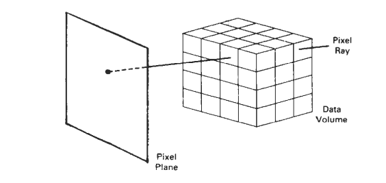
VISUALIZATION OF DATA SETS

Visualization of data sets is a crucial aspect of data analysis and exploration, allowing us to gain insights and understand complex information in a visual and intuitive manner. Data visualization techniques transform raw data into visual representations, such as charts, graphs, maps, and interactive visualizations, enabling us to identify patterns, trends, correlations, and outliers.

Data visualization plays a vital role in various fields, including scientific research, business analytics, finance, healthcare, and many others. It helps communicate information effectively, make informed decisions, and uncover hidden insights within data sets. Here, we delve into the importance, methods, and benefits of visualizing data sets.

Importance of Data Visualization:

1. Simplifying Complexity: Data sets often contain vast amounts of information that can be challenging to comprehend in raw form. Visualization simplifies complexity by presenting data in a visual format that is easier to understand and interpret.
2. Pattern and Relationship Recognition: Visual representations enable us to identify patterns, trends, and relationships between variables. By visualizing data, we can quickly spot correlations, clusters, or anomalies that may not be apparent in raw data.
3. Storytelling and Communication: Visualizations enhance storytelling by presenting data in a compelling and accessible manner. They enable effective communication of insights, making it easier to convey complex information to diverse audiences.

Methods of Data Visualization:

1. Charts and Graphs: Bar charts, line charts, scatter plots, pie charts, and histograms are common graphical representations used to visualize data sets. They provide a concise summary of data and facilitate comparisons, distributions, and trends.
2. Maps and Geospatial Visualizations: Geographical data can be visualized using maps and geospatial visualizations. Heatmaps, choropleth maps, and interactive map interfaces are effective in displaying spatial patterns and regional variations.
3. Network Visualizations: Network visualizations depict relationships between entities using nodes (vertices) and links (edges). They are used to analyze social networks, transportation networks, and complex systems, helping us understand connections and interactions.
4. Interactive Visualizations: Interactive visualizations allow users to explore and interact with data. They provide functionalities like filtering, zooming, and drill-down, enabling users to dive deeper into specific aspects of the data set and gain more insights.

Benefits of Data Visualization:

1. Data Exploration: Visualization facilitates data exploration by allowing users to interactively navigate and analyze the data from different angles, revealing new perspectives and insights.
2. Rapid Insight Generation: Visual representations provide an efficient way to generate insights quickly. Patterns, outliers, and trends become apparent at a glance, accelerating the decision-making process.
3. Improved Decision Making: Visualizations enable better-informed decision making by presenting data in a visual context that is easier to comprehend. They help stakeholders understand complex information and make data-driven choices.
4. Enhanced Data Sharing: Visualizations promote effective data sharing and collaboration. They provide a common visual language for discussing and sharing insights, fostering a deeper understanding among team members and stakeholders.

In conclusion, visualization of data sets is a powerful tool for understanding and interpreting complex information. By employing various visualization techniques, we can simplify data, recognize patterns, and communicate insights effectively. Data visualization is indispensable for gaining a deeper understanding of data and making informed decisions across a wide range of domains.

Three Dimensional objects representation in C

Representing three-dimensional objects using C programming involves utilizing appropriate data structures and algorithms to store and manipulate the object’s geometry, topology, and attributes. Here is a general outline of how three-dimensional objects can be represented using C:

1. Vertex Representation:
   Start by defining a structure to represent a vertex in three-dimensional space. Each vertex consists of three coordinates (x, y, z) that define its position. You can create a struct in C to hold these coordinates, such as:

struct Vertex {
    float x;
    float y;
    float z;
};

2. Mesh Representation:
   To represent a three-dimensional object composed of polygons, you need to define a data structure to store the connectivity information of the vertices. One common representation is to use an array of vertices and an array of indices that define the connectivity between them. For example:

struct Mesh {
    struct Vertex* vertices; // Array of vertices
    unsigned int* indices;   // Array of vertex indices
    unsigned int vertexCount; // Number of vertices
    unsigned int indexCount;  // Number of indices
};

3. Object Attributes:
   You may also want to include additional attributes for each vertex, such as vertex normals, texture coordinates, or vertex colors. These attributes can be stored alongside the vertex coordinates in the Vertex structure or in separate arrays, depending on the complexity of the object representation.
4. Operations and Algorithms:
   Implement various operations and algorithms to manipulate and process the three-dimensional object. This may include functions for loading and saving object data from files, transforming objects (e.g., translation, rotation, scaling), performing geometric calculations (e.g., surface area, volume), and rendering the object using graphics APIs or libraries.
5. Memory Management:
   Ensure proper memory management to allocate and deallocate memory for the vertices, indices, and any additional attributes. You may need to write functions to create, destroy, and resize the mesh data structure, taking care of memory allocation and freeing resources when they are no longer needed.
6. Usage and Integration:
   Integrate the object representation into your application or system, allowing users to interact with the 3D object, apply operations, and visualize or process it according to your requirements.

Remember that this outline provides a general approach to represent three-dimensional objects in C. The specific implementation details will depend on the complexity and requirements of your application. Additionally, there are various libraries and frameworks available in C that provide more advanced features for 3D object representation and manipulation, such as OpenGL, DirectX, or third-party libraries like OpenMesh or Assimp, which can simplify the process and provide additional functionality.