Applications of Hoffman coding in data compression

Top Applications of Hoffman coding

Lossless Image Compression

A simple application of Huffman coding to image compression would be to generate a Huffman code for the set of values that any pixel may take. For monochrome images, this set usually consists of integers from 0 to 255. Examples of such images are contained in the accompanying data sets.

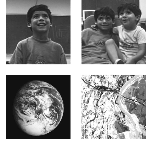
Compression using Huffman codes on pixel difference values

Image Name	Bits/Pixel	Total Size (bytes)	Compression Ratio
Sena	4.02	32,968	1.99
Sensin	4.70	38,541	1.70
Earth	4.13	33,880	1.93
Omaha	6.42	52,643	1.24

Compression using adaptive Huffman codes on pixel difference values

Image Name	Bits/Pixel	Total Size (bytes)	Compression Ratio
Sena	3.93	32,261	2.03
Sensin	4.63	37,896	1.73
Earth	4.82	39,504	1.66
Omaha	6.39	52,321	1.25

Text Compression

Text compression seems natural for Huffman coding. In text, we have a discrete alphabet that, in a given class, has relatively stationary probabilities. For example, the probability model for a particular novel will not differ significantly from the probability model for another novel. Similarly, the probability model for a set of FORTRAN programs is not going to be much different than the probability model for a different set of FORTRAN programs. The probabilities in Table 3.26 are the probabilities of the 26 letters (upper- and lowercase) obtained for the U.S. Constitution and are representative of English text. The probabilities in Table 3.27 were obtained by counting the frequency of occurrences of letters in an earlier version of this chapter. While the two documents are substantially different, the two sets of probabilities are very much alike..

T A B L E 3 . 26

	Letter	Probability		Letter	Probability
	A		0057305			N	0.056035
	B		0014876			O	0.058215
	C		0025775			P	0.021034
	D		0026811			Q	0.000973
	E		0112578			R	0.048819
	F		0022875			S	0.060289
	G		0009523			T	0.078085
	H		0042915			U	0.018474
	I		0053475			V	0.009882
	J		0002031			W	0.007576
	K		0001016			X	0.002264
	L		0031403			Y	0.011702
	M		0015892			Z	0.001502
	T A B L E 3 .27
	Letter	Probability		Letter	Probability
	A	0049855			N	0.048039
	B	0016100			O	0.050642
	C	0025835			P	0.015007
	D	0030232			Q	0.001509
	E	0097434			R	0.040492
	F	0019754			S	0.042657
	G	0012053			T	0.061142
	H	0035723			U	0.015794
	I	0048783			V	0.004988
	J	0000394			W	0.012207
	K	0002450			X	0.003413
	L	0025835			Y	0.008466
	M	0016494			Z	0.001050

Text Compression

Text compression seems natural for Huffman coding. For example, the probability model for a particular novel will not differ significantly from the probability model for another novel. Similarly, the probability model for a set of FORTRAN programs is not going to be much different than the probability model for a different set of FORTRAN programs.

Audio Compression

Another class of data that is very suitable for compression is CD-quality audio data. The audio signal for each stereo channel is sampled at 44.1 kHz, and each sample is represented by 16 bits. This means that the amount of data stored on one CD is enormous. If we want to transmit this data, the amount of channel capacity required would be significant. Compression is definitely useful in this case. In Table 3.28 we show for a variety of audio material the file size, the entropy, the estimated compressed file size if a Huffman coder is used, and the resulting compression ratio.